The following steps need to be done for getting the gm/Id vs Id/(W/L) graphs in Cadence for a MOS transistor.
Create the schematic
The schematic is a simple transistor schematic. The schematic below shows an example:
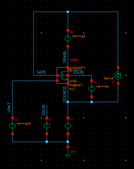
The above schematic shows that the drain current(di), vgd, vbs, W and L are parameterized and they are sweeped in the simulation script (except vbs) to get the graphs for a wide range of conditions and check the variation of the graph for them.
Save Operating Point Info
Create a text file called
mysaves_t18.scs and add the following line in it:
Now add this file with path in ADE->Setup->Simulation Files->Definition Files
Note that the .m0 is only needed because this model is implemented as s Sub Circuit in the models file. If the model is not a subcircuit and something direct like a BSIM model then .m0 would not be needed.
Setup simulation in ADE
Setup the DC sweep simulation in ADE by DC sweeping di from a low value to a high value for a typical vgd, W and L. Set the sweep to be logarithmic with 50 points per decade. Also setup expressions to calculate
- gm/Id = gm/di expression: (getData("MNO_PSP.m0:gm" ?result "dc-dc")/IS("/V1/PLUS"))
- Id/(W/L) expression: (IS("/V1/PLUS")/(5e-6/180e-9))
Run the Simulation and see the results.
Create the Ocean Script
Save the Ocean Script from the ADE environment and modify it to look like the following:
- ; Select the waveform tool
- ocnWaveformTool( 'wavescan )
-
- ; Select the simulator
- simulator( 'spectre )
-
- ; Specify the Design Netlist
- design( "/sim/mgupta/nch_char_1/spectre/schematic/netlist/netlist")
-
- ; Specify the Results Directory
- resultsDir( "/sim/mgupta/nch_char_1/spectre/schematic" )
-
- ; Specify the model files set
- modelFile(
- '("/home/tekcad/cds4_4/lib/models.scs" "tt_res")
- '("/home/tekcad/cds4_4/lib/models.scs" "tt_mim")
- '("/home/tekcad/cds4_4/lib/models.scs" "tt")
- )
-
- ; Specify the Definition file created to save the operating point
- definitionFile(
- "/home/mgupta/Cadence/mysaves_t18.scs"
- )
-
- ; Convert the main run steps to a procedure 'mysim' and convert width, length, vgd, istart, istop
- ; etc as variables to be passed along with the filehandle where to write the results
- procedure(mysim(istart istop length width vgd fileHandle)
- analysis('dc ?param "di" ?start istart ?stop istop ?dec "50" )
- desVar( "l" length )
- desVar( "vgd" vgd )
- desVar( "di" 5u )
- desVar( "w" width )
- save( 'i "/V1/PLUS" )
- temp( 27 )
- run()
- gm_by_Ids = (getData("MN0_PSP.m0:gm" ?result "dc-dc") / IS("/V1/PLUS"))
- id_by_w_l = IS("/V1/PLUS")*length/width
-
- ;Comment out the plot statement
- ;plot( gm_by_Ids ?expr '( "gm_by_Ids" ) )
-
- ; Write the results in the filehandle
- ocnPrint( ?output fileHandle ?numberNotation 'engineering ?numSpaces 10 id_by_w_l gm_by_Ids)
- )
-
- ; Create file for writing the results
- resultFile = outfile( "./Curves/gmByIdCurves.csv" "w")
- ; Close the file
- close(resultFile)
-
- ; Lists for iterating the simulation
-
- length_list = list(180e-9 500e-9 1e-6 1.5e-6 2e-6 2.5e-6 3e-6 3.5e-6 4e-6 4.5e-6 5e-6 5.5e-6 6e-6 6.5e-6 7e-6 7.5e-6 8e-6 8.5e-6 9e-6 9.5e-6 10e-6)
- ;length_list = list(180e-9 500e-9)
- width_list = list(2e-6 4e-6 6e-6 8e-6 10e-6 15e-6 20e-6)
- ;width_list = list(2e-6 4e-6)
- vgd_list = list(0.3 0 -0.3 -0.6 -0.9)
- ;vgd_list = list(0.3 0)
-
- min_IdbyWL = 1e-9
- max_IdbyWL = 200e-6
-
- ; Loop through all the lists
- foreach( vgd vgd_list
- foreach( width width_list
- foreach(length length_list
- ; Calculate istart, istop so that Id/(W/L) starts and stops the same for every W/L combination
- istart = min_IdbyWL*width/length
- istop = max_IdbyWL*width/length
- ; Write the data in a temp File
- tempFile = outfile("./Curves/gmByIdtmp.out" "w")
- mysim(istart istop length width vgd tempFile)
- ; Close the file
- close(tempFile)
- ; Combine the data file and temp file to an intermediate file
- ; Create the intermediate file
- system(sprintf(nil "pr -mr -t -s\\ %s %s > %s" "./Curves/gmByIdCurves.csv" "./Curves/gmByIdtmp.out" "./Curves/gmByIdinter.out"))
- ; remove the Curves data file
- system(sprintf(nil "rm -rf ./Curves/gmByIdCurves.csv"))
- ; rename intermediate file to Curves file
- system(sprintf(nil "mv ./Curves/gmByIdinter.out ./Curves/gmByIdCurves.csv"))
- )
- )
- )
-
- ; Remove the temporary File
- system(sprintf(nil "rm -rf ./Curves/gmByIdtmp.out"))
Save this ocean script (say 'gmByIdScript.ocn') and load it from the CIW window by typing:
This would start the simulations and at the end we would have the file gmByIdCurves.csv with all the simulation results.
Draw the Graph using MATLAB
Finally create the following script in MATLAB and name it
mergeGraphs.m and run it to create the graphs in a figure:
- % Script to read gmbyId.txt and merge the readings to just 1 graph
- % 1st column is taken as Current, 2nd column as Id/(W/L), 3rd column as
- % gm/Id
- % Remove the 1st 2 lines as the header lines
-
- arr = textread('gmByIdCurves.csv','',-1,'headerlines',2,'headercolumns',0);
-
- figure(1);
- for count = 2:3:size(arr,2)
- semilogx(arr([1:size(arr,1)],count),arr([1:size(arr,1)],count+1),'r');
- hold on;
- end
- grid on;
-
- xlabel('Id/(W/L)')
- ylabel('gm/Id')
- title('gm/Id vs Id/(W/L) for 2V NMOS TSMC 0.18\mum RF; 180nm \leq L \leq 10\mum, 2\mum \leq W \leq 20\mum, 0.3V \leq Vgd \leq -0.9V')
Drawing the Graph using gsl-shell
Use the following script. The script can be loaded in gsl-shell using the command dofile('script_path_and_name').
- csv = require 'csv'
- t=csv.read('MyScripts/gmByIdCurves.csv')
- -- Convert it to a 2D numeric array since the csv is space separated and not "," separated
- curves = {}
- for i = 4,#t do
- curves[#curves+1] = {}
- for n in string.gmatch(t[i][1],"%S+") do
- curves[#curves][#curves[#curves]+1] = tonumber(n)
- end
- end
-
- -- Now all the data table is in Curves:
- -- 1st column is drain current
- -- 2nd column is Id/(W/L)
- -- 3rd column is gm/Id
- -- And it repeats
- p = graph.plot()
-
- for i = 2,#curves[1],3 do
- -- Create the line here
- ln = graph.path(math.log10(curves[1][i]),curves[1][i+1])
- for j = 2,#curves do
- ln:line_to(math.log10(curves[j][i]),curves[j][i+1])
- end
- p:addline(ln)
- end
- p:show()
Sample Graph
Shown below is a sample graph from the above steps:
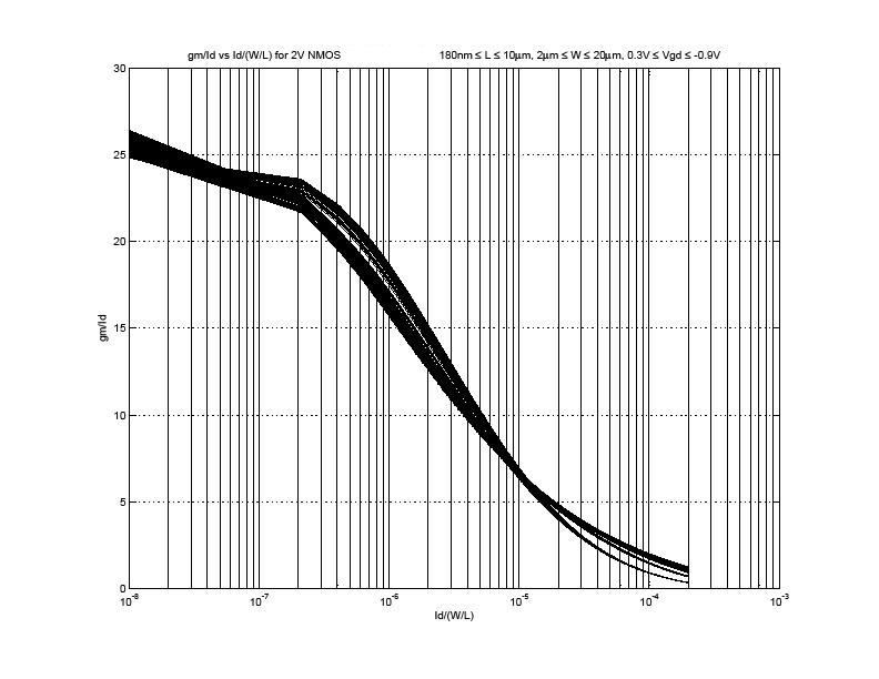
NOTE This graph was taken with a linear sweep a better graph will result of the sweep is set to logarithmic especially with no discontinuity in the slope as it seems in this one.
References