Concepts

[top]

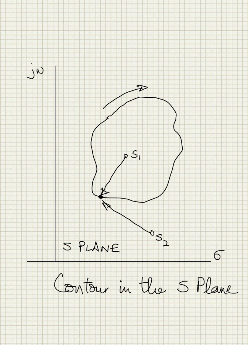
1. If we visualize all the poles and zeroes of the loop gain on the s-plane and draw any closed contour anywhere in the s-plane. If we traverse the contour in the clockwise direction then the net change in phase of the phasor from a zero inside the contour is -360 deg (-2 pi radians). For a pole it will be +360 deg (+2 pi radians). The sign of the phase change for zero is negative and for pole is positve because zero terms are in the numerator of the transfer function while poles are in the denominator and we make the traversal in the clockwise direction which is the negative direction of phase change on the s plane. Note that the sign is the artifact of the direction of traversal. For any pole/zero outside the contour the net change of the phase of the phasor is 0 always. See image below:

   

2. Therefore net change in phase for a clockwise traversal on any s-plane contour is

   2 pi (P-Z) radians 
              where P=number of poles in the contour 
              and Z=number of zeroes in the contour
   

3. Now plot this contour (the contour that we just traversed in the above step in the s plane) in a plane with the x value as the real part of the net phasor from all the poles and zeros and the y values as the imaginary part of the net phasor from all the poles and zeros. This seems a bit complicated to get since we have to claculate the phasor from all poles and zeros and then take the real and imaginary parts. However getting this is not that difficult since the net phasor is the loop gain if we choose the contour running all the way on the imaginary axis of the x plane. So this new plane is essentially the net phasor plane. Lets call it the F(s) plane i.e the plane of the contour phasor function.

   NOTE: The 'net phasor' is the phasor representing the net phase change when we add the phase change contributions of traversing the contour for the phasor from every pole and zero of interest so which is the same as the phasor for the pole zero polynomial. It is not the addition of all phasors from all the poles and zeros since that does not give the net effect of the phase change but produces a phasor with its own new phase. For example:

   

   Here there is pole at 1,-1 and zero at 2,-2 and we are considering a point 2,-1 as a point on the contour. So the addition of the 2 phasors from the singularities has a magnitude $√2$ and phase of pi/4 which is very different than the polynomial phasor which is given as:

   $${s-(2-j2)}/{s-(1-j)}$$

   and if we put s=2-j we get

   $${(2-j)-(2-j2)}/{(2-j)-(1-j)}=j$$

4. Now if the phase of certain phasors (considering a phasor from each singularity to the contour) change by 2 pi (P-Z) and some phasors remain the same the net change in the phase for the clockwise traversal of the contour is also 2 pi (P-Z). The phase increase in the F(s) plane is simply an encirclement of the origin (remember this plane is just the F(s) phasor plotted directly!) in the clockwise direction for every 2 pi radian phase increase.
   1. If the contour encircles a zero the F(s) plane contour will encircle the origin clockwise
   2. If the contour encircles a pole the F(s) plane contour will encircle the origin anti-clockwise
   3. If the contour encircles equal poles and zeroes or does not encircle a pole/zero then the contour in F(s) will not encircle the origin.

   This is shown below in the 2 examples. The 1st example has a zero in the s plane and the contour encircles it so the contour in the F(s) plane goes around the origin. In example 2 the zero is outside so the F(s) plane contour does not encircle it.

   

   

   Let us look at an example with numbers to convince ourselves of this. Consider a singularity at 1,1 in the s plance and the contour we trace around it be going from 0,0 to 0,2 to 2,2 to 2,0 to 0,0 i.e a square going clockwise. As shown in the diagram below:

   

   if the singularity is a zero then the corresponding point in the F(s) plane can be calculated by considering that F(s) = s-(1+j) and substituting the value of s for the 4 corners of the square clockwise contour. With that we get the diagram below, which shows that for a clockwise encirclement of 0 we encircle the origin in the F(s) plane in the clockwise direction:

   

   Doing the same thing by considering the singularity a pole we have F(s) = 1/(s-(1+j)) and we can trace out the following diagram showing that to encircle a pole in the s-plane results encircling the origin in the F(s) plane in anticlockwise direction:

   

5. If we define P(s) = F(s) - 1 so that F(s) = P(s)+1 then P(s) is just the F(s) curve shifted by 1 to the left. So if F(s) encircles 0 then P(s) encircles -1. This point relates the loop gain with the denominator of a closed loop system. So all the Nyquist criteria will check is that 1+Loop Gain should not have any right half plane zeros since they are the right half plane poles of a closed loop transfer function and hence make the system unstable.

Applying to Stability

[top]

1. The loop gain can be considered a partial contour extending from -j inf to + j inf. We can close the contour by creating a semi circle on the RHP of the s-plane with a radius of infinity. So now we have a contour that encircles the entire RHP
2. Stability requirement for the system G(s)/(1+G(s)H(s)) is that this system should not have any right half plane poles. G(s)H(s) is the loop gain. Thus the 1+G(s)H(s) function should not have zeroes in the right half plane. So if the mapping of the Loop gain (G(s) H(s) ) contour encircles -1 in clockwise direction, it means that 1+G(s)H(s) encircles origin in clockwise direction and then we have right half plane zero which is a right half plane pole for the full system and hence will cause instability because normally there should be no right half plane poles in the loop gain.
3. Since Re[G(jw)H(jw)] = Re[G(-jw)H(-jw)] i.e. Real part is even and Im[G(-jw)H(-jw)] = -Im[G(jw)H(jw)] i.e. Imaginary part is odd we can just plot the curve for the w values 0 to + inf and just reflect it on the real axis to get the full nyquist plot.
4. Plotting the mapping of the infinite radius circle of the s-plane may require taking limits to find the mapped points in the F(s) plane. See Valkenburg reference examples.

Example

[top]

Now let us see with an example how we handle the contour at infinite and also test the concept by changing the contour and see if we get what we expect. Let:

here $s=σ+jw$ so if G(s) is out loop gain it has a pole at s=-1
Now for stability 1+G(s) should not have any right half plane zero i.e. with a contour enclosing the RHP in the clockwise direction 1+G(s) should not encircle the origin in the clockwise direction or simply G(s) should not encircle the point -1,0 in the clock wise direction. The contour on the S plane is:


Also $G(jw)={1-jw}/{1+w^2}$. As it is clear from this that for any point on the jw axis the Real part of G(jw) > 0 so it is always on the right half plane of the G(s) plane. Now let us see the trace for the semicircle at infinity in the right half s plane:

$r→∞$ so $G(re^{jθ}) = 1/re^{jθ}>0$
So the locus of the contour on the G(s) plane remains on the right side and never crosses the imaginary axis hence it can never encircle zero which is what we expected since the contour never enclosed any pole or zero. So the G(s) plane contour does not encircle -1.
Now let us consider what we should expect to see if we encircle the Left half s plane in a contour and trace it on the G(s) plane. The contour looks like:

For this contour we expect that the G(s) plane contour should encircle the origin once in counter clockwise direction. Let us start on the contour from the origin and go down the jw axis and create a table of values as we go down to see the trend:

s	Re[G(s)]	Im[G(s)]
0	1	0
-j3	0.1	0.3
-j33	9.174e-4	0.03027
-j333	9.018e-6	3.003e-3

So we see that we start from 1,0 and then move towards the top and left in the G(s) plane that is the anticlockwise direction until we reach very close to 0 when w becomes very large. Now to encircle the origin we must have some point where Re[G(s)] = 0 and that happens for $σ=-1$. So it does cross over. To see the effect of the semicircle at infinite let us represent G(s) in polar form. So we have:

$r→∞$ so $G(re^{jθ}) = 1/re^{jθ} = e^{-jθ}/r$
So the phase of G(s) varies from $-3π/2 to -π/2$ which is going in the anticlockwise direction around the origin. And then the jw axis coming from infinite back to origin it just mirrors its path from origin to 1,0. So we have the following G(s) contour:

Interesting Result

[top]

• I can have a stable system with my main amplifier having a right half plane pole

Main amp G(s) = 1/(s-0.5)
H(s) = 1
Vo/Vi = 1/(s+0.5) which is stable!

• Issue is that it creates a Right half plane zero which will cause stability problems and only looking for clockwise encirclements of -1,0 is not enough.

References

[top]

1. See Network Analysis by M.E. Valkenburg Chapter 16: Stability in feedback systems for a good analysis of Nyquist criteria.

1. Nyquist Plot in Cadence